
 Kurtosis Samples
In addition to quantitative metrics such as zero-to-peak, peak-to-peak, and RMS, it is possible to extract metrics regarding the shape of a waveform signal.
Since a digital signal is made up of discrete points in time, we can treat any vibration signal as a statistical distribution of acceleration points.
Vibration signals and the Gauss Curve
You have probably heard of the normal, or Gaussian, distribution. This is one of the most widely used probability distributions for modelling natural phenomena.
Analyzing the following figure, the widest range of this distribution, corresponding to 3 sigmas, represents about 99.74% of the values of a signal. This region is known as the natural range of variation of the process.

In statistics, it is understood that a process always has a certain degree of variability, that is, it operates within a range of values, with a certain variation. If the process is stable, that means that the variation will occur within this range of values.
Applying this concept to machine vibration, if we have a random signal in acceleration, we will have a normal distribution similar to the following:


Kurtosis
The metrics of Kurtosis (also translated as distortion) is an important statistical parameter. This parameter is used to qualitatively describe the shape of a vibration signal.
In the context of vibration analysis, this parameter is used to quantify the peaks of a signal, as well as the degree of symmetry around its mean value.
The kurtosis in a vibration signal can be interpreted graphically by looking at the distribution of the signal values, as shown in the lef figure.
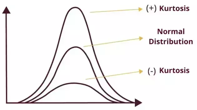
The distribution shape of a signal with a normal or random distribution, as showed earlier, has a kurtosis value equal to 3.
A distribution with a higher kurtosis will have a more tapered shape, with a concentration of values around its mean. On the other hand, a distribution with a lower kurtosis will have a flat shape, with values spread over a larger range.
Shortly, kurtosis expresses how similar the values of a signal are. Therefore, in case of a signal with many distinct peaks or impacts, the kurtosis will be higher.
Let’s look at some examples:
In a new bearing, due to the lack of defects, a rather random signal is expected, such as the one shown in the following waveform. In this case, the kurtosis value will be close to 3.


As defects in a bearing emerge and evolve, the impact signals directly modify signal distribution, this leads to a change in the kurtosis value. As we can see below, the signal has a high kurtosis value of 10.

In all cases, from the waveform, it is possible to extract the kurtosis in terms of acceleration, velocity, displacement, and envelope, making the analysis even richer and more pertinent.
More examples of kurtosis applications
Time comparisons are also valid for identifying defect evolutions. Take the following example, an exciter of a vibrating screen that had a bearing defect (inner race), as illustrated in the spectral envelope below:

When we look at the kurtosis metric in time acceleration for this monitoring point, focusing on a high frequency band (1000 Hz to 6400 Hz) we see that the value has increased significantly. As the bearing defect evolves, we can notice the increased presence of peaks in the waveform signal.

It is important to emphasize that these waveform parameters do not replace spectral analysis; in fact, they are complementary. The best vibration analysis will therefore be done by crossing all techniques for a better diagnosis.